For optimization problems, a solution space contains every possible solution given a set of parameters. If you’ve worked with optimization problems before, you’ve likely seen visualizations depicting these spaces as landscapes resembling Earth’s terrain, like mountains and valleys, but in higher dimensions. Solving an optimization problem means finding the highest peak in this high-dimensional landscape. Genetic algorithms are a common tool for this task.
I wondered if anyone had ever seen what solution spaces actually look like. So I came up with the idea to plot one, pixel by pixel. Obviously, that's not feasible when dealing with a large number of dimensions. Not only would it take too long to calculate the fitness of every solution, but you can only visualize up to three dimensions on a screen at once without distortion. A brute-force approach like this is only feasible if applied to at most three parameters at a time.
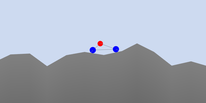
To test this idea, I designed an optimization problem involving a car driving on rough terrain in a 2D environment. The car consists of three circular bodies: two wheels and a red chassis. The goal is to optimize the chassis’s position (XY coordinates) and radius to maximize how far the car travels within a fixed time. The terrain is randomly generated and remains consistent across all trials. If the chassis collides with the terrain, the fitness is determined by how far the car had driven up until that point.
The three parameters are:
To visualize the solution space of these parameters, I need to map every combination of values to a pixel in a 2D texture sequence. The first two parameters define the pixel’s XY coordinates, while the third corresponds to texture depth. Pixel color represents fitness score (brighter = better).
Starting small, I first brute-forced a 32x32 grid of chassis XY positions. The chassis position is restricted to the area just above and between the wheels. The third parameter is ignored for now. The video above shows each solution being tested sequentially, with fitness written to the texture on the left. After brute forcing all solutions, it shows the best solution it found. The fitness texture on the left shows an undistorted visualization of this solution space, albeit at low resolution.
Adding the third parameter (chassis radius) expands the solution space to three dimensions. The 3D solution space is visualized in the video seen above, where each frame represents a continuous variation in the chassis radius. The chassis radius starts smaller than the wheels in the first frame and gradually increases to slightly larger than the wheels by the final frame. The video has a resolution of 512x512 which allows us to see in detail just how complex this multidimensional landscape is. Just look at all that complexity! It looks strangely fascinating.
To make sense of the above video in simple terms: It shows you how large the chassis should be and where the chassis should be placed in order to get the best possible score for the car.
In the video above, we see a more "zoomed out" view. Out of curiosity, I allowed the chassis position to be placed much farther away from the wheels, even so far away that it could intersect with the terrain. That's why you can see a bit of terrain inside this solution space. Surprisingly, many of these pixels scored well despite seeming impractical. Why would placing the chassis underneath the terrain or far up in the sky score highly?
To find out why the fitness scores were so high for seemingly impractical cars, I selected two bright pixels in odd locations to see how those cars performed. As it turns out, it's because placing the chassis far enough away causes the joints to behave erratically.
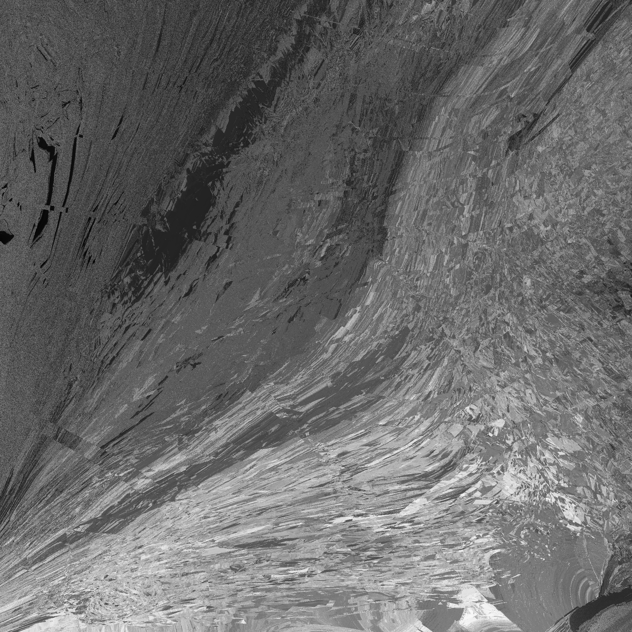
The above image is a 2048x2048 resolution visualization of the solution space for the first two parameters (chassis XY position). In this case, the car is invincible, meaning it can continue driving even after the chassis collides with the terrain. This causes the texture to appear brighter, as it helps the car drive even farther. Click the image to view it in full size. Each pixel in the image represents a unique car.
We’ve now seen what complex solution spaces can look like. I think the results are interesting. These solution spaces appear far more complex and less smooth than I expected. Maybe the rough terrain is to blame? I can imagine how difficult it would be for a genetic algorithm to find the brightest pixel in any of these solution spaces.
You can find the source code of this project Here.